
Make use of our RBSE Class 12 Accountancy Notes here to secure higher marks in exams.
Rajasthan Board RBSE Class 12 Accountancy Notes Chapter 13 Application of Electronic Spreadsheet in Accounting
Introduction of Excel
Excel is the spreadsheet program created by Microsoft. Although you can use any spreadsheet program for analysing data, the instructions given here are specific for Excel and you must use Excel for the three excel quizzes.
Note: Microsoft also makes a less powerful spreadsheet program as part of Microsoft works or some similar title.
Some of the features that we will use in these exercises are not found in MS works so you will not be able to complete all the exercises using MS works.
Excel is in its most basic form a very fancy calculator. The information given in this quick tutorial is meant to give a working knowledge of how to use Excel. There are usually several different ways to perform the same function in Excel, this tutorial will usually just give one way.
If you need more information on how to use Excel there are many websites dedicated to using Excel, a simple “Google” search will find many of them. In addition accessing the HELP menu from within the program can also be useful.
It is a versatile program present on most computers at home and in computer clusters. It is a business tool for accounting and managing large sets of data. It can also simplify graphing and analysing data from the labs. These instructions are intended as a guide to graphing lab data for those who are not familiar with excel.
As always with computer program there is more than one way to go about these things. The instructions here are intended to be an easy introduction to the use of excel.
Interface
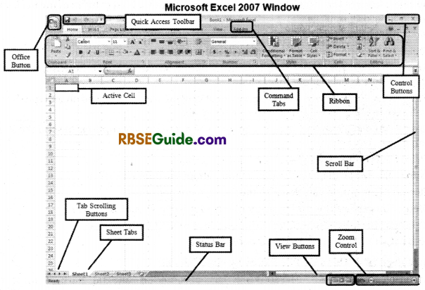
The first figure shows the typical Excel sheet with the important parts of the programs interface labelled.
![]()
1. Back Stage View in Excel
The back stage view has been introduced in Excel 2010 and acts as the central place for managing your sheets. The backstage view helps in creating new sheets, saving and opening sheets, printing and sharing sheets and so on.
Getting to the back stage view is easy. Just click the file tab located in the upper left corner of the excel ribbon. If you already do not have any opened sheet then you will see a window listing down all the recently opened sheets.
If you already have an opened sheet then it will display a window showing the details about the opened sheet as shown below. Back stage view shows three columns when you select most of the available options in the first column. First column of the back stage view will have the following options.
- New: This option is used to open a new sheet.
- Open: This option is used to open an existing excel sheet.
- Save : If an existing sheet is opened it would be saved as it is, otherwise, it will display a dialogue box asking for the sheet name.
- Save As : A dialogue box will be displayed asking for sheet name and sheet type. By default it will save in Sheet 2010 format with extension, xlsx.
- Save & Send: This option saves an opened sheet and displays options to send the sheet using email, etc.
- Print: This option is used to print an opened sheet.
- Info: This option displays the information about the opened sheet.
- Recent: This option lists down all the recently opened sheets.
- Help; You can use this option to get the required help about Excel 2010.
- Options: Use this option to set various options related to Excel 2010.
- Exit: Use this option to close the sheet and exit.
![]()
2. Importance and Uses of MS Excel Spread Sheet
Microsoft Excel spreadsheet software has become an integral part of most business organisations across the world. MS Excel is used for various purposes by business establishments. Some organisations use this spreadsheet software for generating memos, track sales trends and other business data.
Microsoft Excel spreadsheets software come with million rows of data and automate number crunching, but this popular spreadsheet software is capable of doing more than just figures. MS Excel has a simple interface that allows users to easily understand this software and also perform basic activities.
Ms Excel offers a grid interface that allows the users to organise any type of information they require. One of the major advantages of MS Excel spreadsheet software is its flexibility feature. This feature allows the users to define the structure of information they need to manage with ease and this spreadsheet software is very easy to use and even a notice users can use this software for specialised tasks.
The users needs to undergo training and gain hands on experience to use it in a better manner. Even after three decades, Microsoft Excel is still the most preferred and used spreadsheet software around the world. Microsoft Excel is commonly used for financially related activities.
The reason for its popularity is that the users can define custom formulas for calculating quarterly, half yearly and annual reports. This spreadsheet software also helps the individuals and professionals to effectively keep a track of sales leads, project status reports and invoice reports.
Microsoft Excel is also very popular among professionals from Science background as it allows them to easily work with statistical formulas and graphing. This article offers a brief introduction to Microsoft Excel and its key features.
(i) Work Scheduling : Assigning the work tasks to the team members is one of the most important job of the managers. This task must be performed by managers effectively so that the given project deadlines are met and the project is delivered successfully to the client.
For this manager take advantage of scheduling feature available in the MS Excel spreadsheet software. These schedules can be colour-coded and are designed in such a manner that they get automatically updated if there is a change in the schedule of tasks and activities.
(ii) Basic Financial Accounting : Small and mid-sized organisations make use of MS Excel spreadsheet software for carrying out their accounting activities. They can create a basic accounting program or a larger check book that allows them to keep a track of the organisation’s financial
transactions. For making it more effective accountants can enter their deposits and expenditures onto each row, very much similar as they do it in the traditional ledger books. By entering data in this manner accountants also have the flexibility to create charts and graphs over time to compare business income and expenditure.
(iii) Marketing and Product Management: While marketing and product professionals look to their finance teams to do the heavy lifting for financial analysis, using spreadsheets to list customer and sales targets can help you manage your sales force and plan future marketing plans based on past results.
Using a pivot table users can quickly and easily summarise customer and sales data by category with a quick drag and drop. All part of business can benefit from strong excel knowledge and marketing functions are not exempt.
(iv) Human Resources Planning : While database system like Oracle (ORCL), SAP (SAP) and Quick Books (INTU) can be used to manage payroll and employee information, exporting that data into Excel allows users to discover trends, summarise expenses and hours by pay period, month or year and better understand how your workforce is spread out by function or pay level.
HR professionals can use Excel to take a giant spreadsheet full of employee data and understand exactly where the costs are coming from and how to best plan and control them for the future.
(v) Customer Data : Small business establishments and organisations use MS Excel spreadsheet for storing contact information of their clients and customers. This information acts as customers database for them and can make use of this information to contact their customers.
The advantages of storing this information in MS Excel sheet is that even though the sheet is updated or new fields have been added to the sheet it does not effect or change the content present in other cells of the spreadsheet.
![]()
Inserting Data and Formulas
To insert data you can simply use your mouse to select a cell and then simply type. Start the Excel program. Select the cell A1 (that is the cell in column A, row 1) by using your mouse and clicking the left mouse button (this is the ‘normal’ mouse button). Note that the name of the cell is displayed in the Name Box. By default the name of the cell is its address with reference to the row/column although, you can name a cell anything you w-ant using the Insert/Name menu item.
- Insert the following data into the first 6 rows of the A column
- 56, 67, 76, 55, 62, 69
To do this, simply select the cell (A1 should already be selected) and type in the number 56 and press the enter key. This will insert the number 56 into cell A1 and automatically move the active cell to A2. Now type in 67 into A2, and press enter. Continue in this fashion until all six numbers are inserted in the first 6 rows of column A.
- Insert the following set of numbers into the first 6 rows of column B
- 34, 44, 123, 89, 22, 10
Warning Note: In many instances you will be using numbers with units (like meters or grams) when using Excel, never mix number with letters in a cell. If you do, Excel assumes that you are inserting text and not inserting numbers. For example, if the units for the numbers you inserted in the previous exaihple are grams do not type 34g (or 34 grams) in a single cell.
Excel will not recognise this as a number. Simply type 34. You can use a table on the column to indicate the units. You will learn later how to insert a label. That should have been easy now. Lets do some calculations.
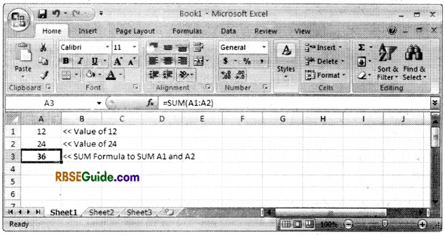
The Hard Way
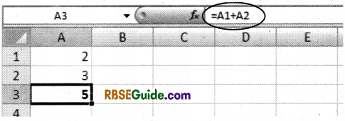
Let’s add the numbers in each column and place the sum in the 7th row of each column. One way (the hard way) would be as follows :
- Select cell A7. This is the cell where the sum will be displayed.
- Type in the equal sign (=). All calculations (or formulas) in Excel must begin with an equal sign.
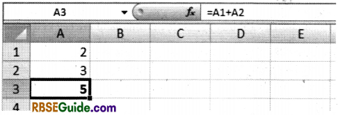
- Type in the arithmetic expression summing the various cells so that the following expression is inserted into the cell = A1 + A2 + A3 + A4 + A5 + A6, and press the ENTER Key. Your sheet should look similar to the following figure :
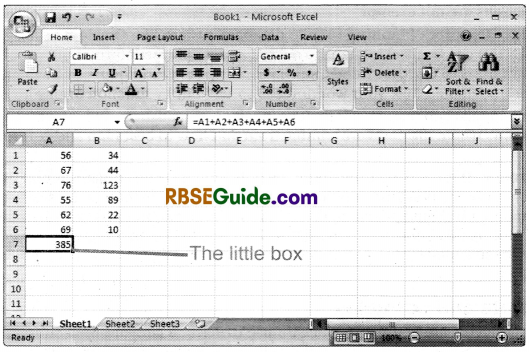
Note that the sum of the numbers in column 1 is displayed in cell 7 and that the formula is shown in the window of the formula bar. If you were to change the value of cell A1 from 56 to 55, you would find that the sum shown in A7 would also change. (Try it, but remember to change it back). NOTE: If you were to forget to start the formula with the equal sign, Excel would assume that you are typing in text and would not do any calculations.
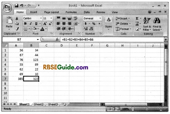
One can do the same procedure to sum the values in column B and type = B1 + B2 + B3 + B4 +B5 +B6 into cell B7 (actually, you could type it into any cell, but it is more logical to use B7). But there is an easier way. Note that there is small box in the lower right corner of any selected cell.
Select cell A7 (as shown above) and move, without pressing a button the corner over the box. You should note that the cursor changes when over the box, changing from a hollow cross to a simple line cross. This will occur automatically whenever the cursor lies over the little box. Do this several times so that you are familiar with its appearance.
Now, with the cursor over the box in cell A7 (and thus in the line format) press down and hold the left mouse button and drag the mouse over cell B7. Once you observe that B7 becomes selected release the button. If done correctly you should find that the formula was copied into B7 but that it summed up the contents of column B7, pretty amazing! Your screen should look like the following figure (with cell B7 selected). This is much easier than typing in all of the cell names into the formula. This process (where you use the little box to copy a formula to adjacent boxes) will be known as “Dragging the Box” in this tutorial.
An Easier Way to Insert a Formula : While the ability to create your own formula in Excel is powerful it is time consuming (not to mention that it requires that you know the formula).
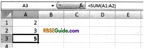
The people at Excel realise this and have created a set of formulas (they call them functions) ready for you to use. There are several hundred predetermined functions in Excel, one of them is the SUM function (which sum a series of cells).
How to Get to SUM : In your spreadsheet select the cell A8. To access the formulas, use the INSERT menu item and select FUNCTION. You should now get the FUNCTION dialog box which is shown below
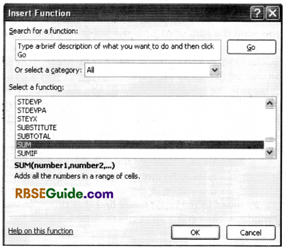
In the category select window (labelled 1 in the figure) select All (as shown). As you become familiar with the different categories, you can use them to make your search a bit easier but for now we know that all the functions will be found in the all category. Scroll down the selection window (section 2) until you reach the SUM function and highlight it with a single mouse click (as shown in the figure).
The functions are sorted in alphabetical order, so you will need to scroll down to the S’s. Note that a brief description of the function is shown in Section 3 of the dialog box. With the SUM function selected, press the OK button. You will now see a new dialog box titled FUNCTION ARGUMENTS. In this dialog box, you will indicate which numbers you want summed. This box is shown below:
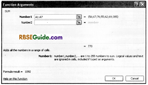
The important section is the input box (number 1 in the figure). As you should see, Excel automatically inputs a range of values that it thinks you want summed. In this case, it is the column of number above the cell containing the function (A8 in this case)-Al : A7. The colon (:) is the Excel convention to indicate all cells between A1 and A7 inclusive. One could also write this by typing all cells individually, but the shortcut is easier.
Note this it is not the range of cells you want to sum as it includes A7 (which is the sum function your previous created) you do not want to include this in the sum. In other words, you want the sum of A1 : A6, use the mouse and click on the first input box (labelled number 1) so that the cursor is blinking to the right of the 7.
Use the backspace to erase the 7 and replace it with a 6. The input box should now read A1: A6 which is the range you want to sum. By the way, suppose you wanted to sum all the numbers in rows 1-6 of both columns (A and B), you can input the B column range in the window “Number 2” by clicking on the window and typing B1 : B6.
You will notice two things after doing this. One is that the sum (shown next to 2 in the dialog box) is now 707 and that a third input window is formed. You can add upto 30 (I think) different input windows. Delete the values, in “Number 2” window, but make sure that the cursor is blinking in that window.
Here is another key to input values into an input window. With the cursor blinking in the “Number 2” window, use your mouse and highlight the cells B1-B6 (highlight by clicking on B1 and drag the cursor down to B6, do not release the mouse button until you reach B6-and do not ‘drag the box’ you do not want to change the values in the cell).
When you finish you will find that the highlighted cells are now included in the input box. I find that this is generally the easiest way to input values into input windows. Now delete all values in “Number 2” and press the OK button. You should find the value in A8 is equal to that in A7. “Drag the box” the copy A8 into B8. Your screen should looks like this :
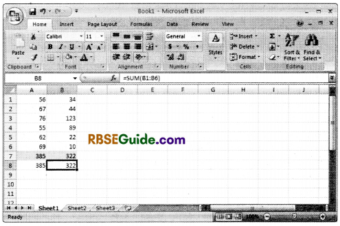
Now the function listed in the formula bar.
Now insert 6 values of your own choosing and place into the first 6 rows of column D. Sum the column in D7 (the hard way) and D8 (the function way). In cell E2, please sum all the values in cells A1-A6, B1-B6 and D1-D6 for a grand total.
Editing the Saving : Your are essentially finished with data manipulation for this EXERCISE. However, the spreadsheet is not clearly labelled. In order to make the sheet easier to understand you will now insert some labels.
Highlight cell Al, use the right mouse button (the one you normally do not use). This will bring up a menu specific for dealing with cells. A example is shown below :
All these menu items deal with cells. Note, any changes you make will only occur on the highlighted cells. In this case the changes will only occur to cell Al. If you highlight several cells and then right click, the changes will occur to all the highlighted one. Also you will find that the right click is a very convenient trick in Excel.
You can right click over almost anything and get a menu specific for that item. It always pays to try it. Play with the various menu items to see what they do. In any case, let Us select the INSERT item.
This will bring up a new dialog box check “entire row” and press OK. This will insert a new, empty row and shift all other rows down 1 row. Insert a column to the left of column A using the same technique, you should now have an empty row 1 and an empty column A.
![]()
Insert Labels: Type “Dogs” into cell B1, “Cats” into cell Cl and “Aardvarks” into cell El. In A8 andA9, type in “Total”. Finally in FI, type, “Total Animals”. By using labels, you can identify what the values in the spreadsheet represent.
Save the File: You are now done with the EXERCISE and must now save the file. From the FILE menu item, select save and complete the dialog box. Name, the file and first initial and last name-my file would be named the xls extension will be added automatically save the file in some place where you will be able to access it, so that you can email the file to your instructor if required.
Spreadsheet: Alternatively referred to as a worksheet, a spreadsheet is a file made of rows and columns that help sort data, arrange data easily, and calculate numerical data. What makes a spreadsheet software program unique is its ability of calculate values using mathematical formulas and the data in cells. A good example of how a spreadsheet may be utilised in creating an overview of your bank’s balance. Below is a basic example of what a Microsoft Excel spreadsheet looks like, as well as all the important features of a spreadsheet highlighted :
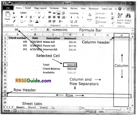
In the above example, this spreadsheet is listing three different cheques, the date their description and the value of each cheque. There values are than added togather to get the total of $162.00 in cell D8. That value is subtracted from the cheque balance to give an available $361.00 in cell D10.
![]()
Uses of a Spreadsheet
Although, spreadsheets are typically used with anything containing numbers, the uses of a spreadsheet are almost endless. Below are some other popular uses to spreadsheets :
Finance: Spreadsheets are ideal for financial data such as your checking accounts information, budgets transactions, billing, invoices, receipts, forecasts and any payment system.
Forms: Form templates can be created to handle inventory, evaluation, performance, reviews, quizzes, time sheets, patient information and surveys.
School and Grades : Teachers can use spreadsheets to track students, calculate grades, and identify relevant data such as high and low scores, missing tests and students who are struggling.
Lists: Managing a list in a spreadsheet is a great example of data that does not contain numbers but still can be used in a spreadsheet. Great examples of spreadsheet lists include telephone, to-do, and grocery lists.
Sports : Spreadsheets can keep track of your favourite player stats or stats’ on the whole team. With the collected data, you can also find averages, high scores and other statistical data. Spreadsheets can even be used to create tournament brackets.
Active Worksheet: An active worksheet is the worksheet that is currently open. For example, in the picture above, the sheet tabs at the bottom of the window show “Sheet 1”, “Sheet 2” and “Sheet 3”, with Sheet 1 being the active worksheet. The active tab usually has white background behind the tab name.
Worksheets Open by Default: In Microsoft Excel and Open OfficeCalc by default there are three sheet tabs that open (Sheet 1, Sheet 2 and Sheet 3). In Google Sheets it starts with one sheet (Sheet 1).
Length Limit of a Worksheet Sheet and Naming : Not to be confused with the file name, in Microsoft Excel there is a 31 character limit for each worksheet sheet name.
Use a Word Processor: While it may be true that some of the things mentioned above could be done in a word processor, spreadsheets have a huge advantage over work processors when it comes to numbers.
It would be impossible to calculate multiple numbers in a word processor and have the value of the calculation immediately appear. Spreadsheets are also much more dynamic with the data and can hide, show and sort information to make processing lots of information easier.
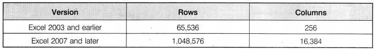
Rows and Columns are In a Spreadsheet
The number of columns and rows supported by a spreadsheet all depend on what spreadsheet program is being used and what version. Below is a list of the maximum number of rows and columns an Excel spreadsheet can have, depending on the version of Excel:
The Excel File/Workbook – Level One
Starting at the highest level you have the Excel Workbook, it will sometimes be referred to as the Excel file as this is basically what it is, your overall Excel file. It depends on who you are speaking to as different users will say phrases like
“Open the Excel file” or “Open the Excel workbook” but if you remember that these terms are interchangeable you won’t go far wrong. The correct terminology is Excel Workbook so this is what we will use from now on.
An Excel Workbook will have a file name, by default a new Excel Workbook will be labelled “Book 1” but as soon as you save the Workbook you will be asked to change the name, ideally this is when you will label your workbook with something more specific so you know what it is. For example, you may call it “Monthly Sales for 2015”.
![]()
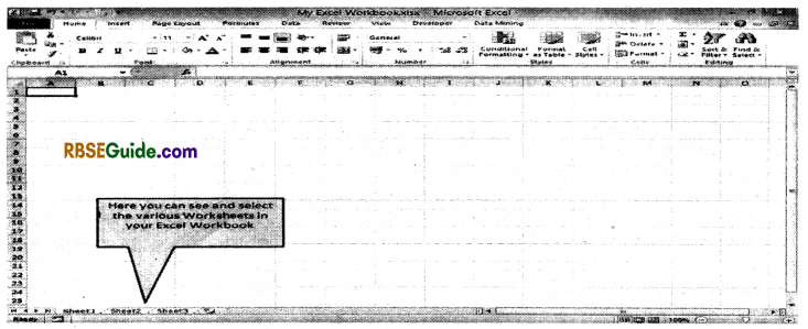
The Excel Worksheet – Level Two
Within every Excel Workbook you must have atleast one worksheet. By default when you create a new Excel workbook it contains three worksheets that are labelled “Sheet 1”, “Sheet 2” and “Sheet 3”. The worksheet is basically your canvas where you complete all your Excel tasks, such as data entry or where you can display tables, charts, shapes, reports and Excel dashboards.
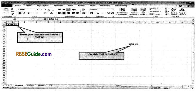
Excel Cells – Level Three
Finally the last level in the basic structure is the Excel Cell. Each worksheet contains lots of cells which you can see in a grid format and each cell will have a unique reference depending on what column and row they are in. For example, the top-left cell in a worksheet is Cell Al because it is in column A and row 1:
Tip: Columns go across the worksheet left to rightand rows go down the worksheet top to bottom. Excel cells are where data can be entered and formulas can be created and the main reason they all have their own unique reference is to assist with calculating formulas or when you get to a more advanced stage, creating Macros and VBA Scripts for automation.
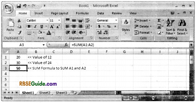
For example, if you have a number in Cell Al and A2 then you can sum those two numbers by using the formula = SUM(A1 \A2), this is useful because if the values in A1 and/or A2 change then your sum will automatically recalculate.
then after the values in Cell Al and A2 have been changed there is no need to redo the SUM formula in Cell A3, it auto-updates with the new total:
Function
A function is a calculation or operation that returns a result. The inputs in a function are called Argumcnts.”
All functions begin with an equal sign [=1. That way Excel knows not to treat the arguments as text. For example, = AVERAGE (2,4) is a function but AVERAGE (2,4) is just a string of text. Without an equal sign, Excel will not calculate a result. The arguments in this function are 2 and 4.
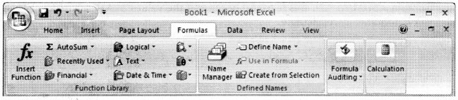
Note, Excel uses upper case letters to list functions. but you can use lower or upper case letters when you write them. In Excel, the “Function Library” can be found on the “Formulas” tab.
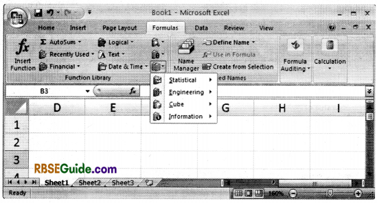
There are 13 categories of functions, some of which are:
- Mathematical : AVERAGE – calculates the average of a series of numbers.
- Date and Time: DATEVALUE – converts a string of text like “30 November 2013” to a number so that you can use this number in other date and time functions. You cannot do maths with dates unless you convert them to numbers first.
- Text: LEN – returns the length of a string. For example, =LEN(”Excel”) is 5.
- Logical: IF – the IF function is vritten like =IF, then A, else B). So, if “test” is true, then the result is A; if “test” is not true, then B.
- Lookup and Reference : These are needed to lookup values elsewhere in the spreadsheet. For example, VLOOKUP looks in a table of values to find one cell.
How could you see that last one? Well, to get the day of the week in text from a date function. You can use VLOOKUP to scan a table to turn this number into something easier to understand, like “Wednesday”.
There are also special functions for financial, engineering and statistics which are listed separately on the “More Functions” menu.
Formula
A formula is combination of “operators”, “operands” and “functions.”
For example, the function = SUM adds a list of numbers (it is so commonly used, that is listed on the first menu, in Excel, abbreviated by the Greek letter Sigma (E:), which is the notation that mathematicians use to sum a series).
You use a formula like doing a calculation by hand. For example, you could put your family budget into a formula like this:
Remaining cash = (4 * weekly salary) – mortgage – food – utilities
The operators are multiply [*] and subtract [-]. The operands are the values “weekly salary”, “mortgage”, “food” and “utilities.” The result is “remaining cash.”
![]()
Names and Addresses
The values for “food” and the other operands are names that you define in Excel. Without a “name”, you would have to use the “address.”
The address of a cell is written using row-column notation. The rows are given numbers and the columns, letters. The first cell in the spreadsheet is Al. When you have reached the end of the alphabet, the rows are numbered AA, AB, BA, BB, and so forth.
Formulas can be more complicated than the family-budget example. In high school you learned that the area of a circle is the radius times pi squared or πr2.
In Excel, you can write this using the formula = PI() * radius Λ2.
Here, PI() is the function that returns the number 3.14 and “radius” is a “name” we have given to a cell that contains the radius; the “operators” are the exponent (A) and multiplier (*).
Order and Precedence
Parentheses are used to indicate the order and precedence in calculations. The area of a circle can also we written πr but not (πr), so you need to understand order and precedence to get right answer. Exponents are evaluated before multiplication, so parentheses are not needed in this case. The function squares the radius first then multiplies that by Pi.
If you wanted to eliminate any possible doubt you could be explicit and write = Pi * (radius Λ2).
![]()
Formulas and Functions
A formula is an expression which calculates the value of a cell. Functions are predefined formulas and are already available in Excel.
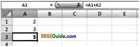
For example, cell A3 below contains a formula which adds the value of cell A2 to the value of cell Al.
For example, cell A3 below contains the SUM function which calculates the sum of the range A1 : A2.
Enter a Formula
To enter a formula, execute the following steps:
1. Select a cell.
2. To let Excel know that you want to enter a formula, type an equal sign (=).
3. For example, type the formula A1 + A2.
Tip: Instead of typing A1 and A2, simply select cell Al and cell A2.
4. Change the value of cell A1 to 3.
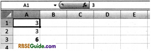
Excel automatically recalculates the value of cell A3. This is one of Excel’s most powerful features.
![]()
Edit a Formula
When you select a cell, Excel shows the value or formula of the cell in the formula bar.
1. To edit a formula, click in the formula bar and change the formula.
2. Press Enter.
Operator Precedence
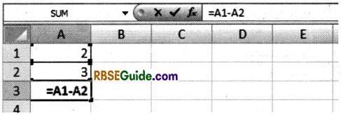
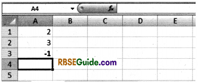
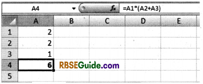
Excel uses a default order in which calculations occur. Ifa part of the formula is in parentheses, that part will be calculated first. It then performs multiplication or division calculations. Once this is complete, Excel will add and subtract the remainder of your formula. See the example below:
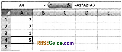
First, Excel performs multiplication (A1 * A2). Next Excel adds the value of cell A3 to this result. Another example,
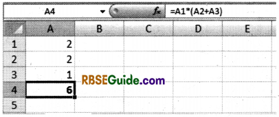
First, Excel calculates the part in parentheses (A2+A3). Next, it multiplies this result by the value of cell A1.
![]()
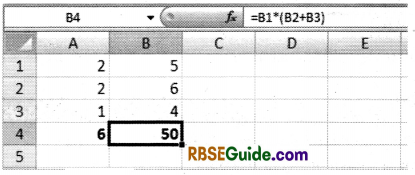
Copy/Paste a Formula
When you copy a formula, Excel automatically adjusts the cell references for each new cell the formula is copied to. To understand this, execute the following steps:
1. Enter the formula shown below into cell A4.
2a. Select cell A4, right click, and then click Copy (or press CTRL + c)…

… next, select cell B4, right click, and then click Paste under ‘Paste Options:’ (or press CTRL + V)

2b. You can also drag the formula to cell B4. Select cell A4, click on the lower right corner of cell A4 and drag it across to cell B4. This is much easier and gives the exact same result.
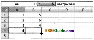
Result : The formula in cell B4 references the values in column B.
Insert a Function
Every function has the same structure. For example, SUM(A1 :A4). The name of this function is SUM. The part between the brackets (arguments) means we give Excel the range Al : A4 as input. This function adds the values in cells Al, A2, A3 and A4. It’s not easy to remember which function and which arguments to use for each task. Fortunately, the Insert Function feature in Excel helps you with this.
To insert a function, execute the following steps:
1. Select a cell.
2. Click the Insert Function button.
The ‘Insert Function’ dialog box appears.
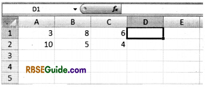
3. Search for a function or select a function from a category. For example, choose COUNTIF
from the Statistical category.
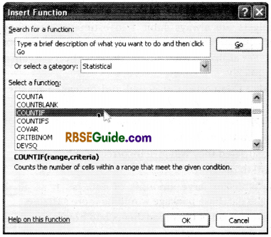
4. Click OK. The Function Arguments’ dialog box appears.
5. Click in the Range box and select the range A1:C2.
6. Click in the Criteria box and type > 5.
7. Click OK.
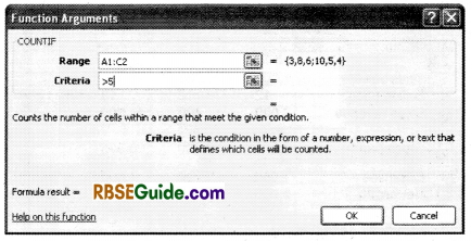
Result. Excel counts the number of cells that are higher than 5.
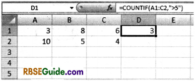
Note: Instead of using the Insert Function feature, simply type = COUNTIF(A1 : C2,”>5″). When you arrive at: = COUNTIF( instead of typing A1 : C2, simply select the range A1 : C2).
![]()
The role of spreadsheet in management accounting, and their advantages and limitations :
Spreadsheets can be used to great advantages in many parts of management accounting. For example,
- Budgeting : Budgets are always subject to estimates and changes. Because formulae automatically update calculations, new budgets can quickly be produced.
- What-if Queries: For example, what-if sales decrease by 5%. Again these experiments can be carried out very quickly.
- Variance Analysis : Comparison of actual and budgeted results and the highlighting of . variances.
Production of Graphics : All spreadsheets allow fast production of graphs and charts. Spreadsheets can be limited in the following areas :
- If incorrectly constructed they will give incorrect results.
- Errors can be hard to discover.
- They are not suitable for large amounts of data, such as all the information held on customers. There, a database package would be more suitable.
![]()
The information that is needed in spreadsheets and how it should be structured :
Apart from labels (descriptions) the information needed in spreadsheets is of three types
- Estimates
- Definite data
- The relationships that hold between pieces of data.
- These three together will produce the results of the spreadsheet. For example,
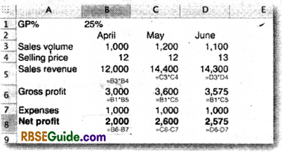
Presumably the sales volumes are estimates. The selling prices and GP% could be definite data (or estimates). The sales revenues and gross profits are calculated data. Here the formulae underlying the numbers displayed are shown in small type in each cell, but the formulae would not be displayed like this on a real spreadsheet.
Rules for Structuring the Data
- Never enter the same figure more than once. So here, the GP% is recorded once only. That means it will be consistently used and will be easy to change.
- Do not type in any figure that could be calculated from others on the spreadsheet.
- Ensure the data is well-labelled so that it is understandable.
Information is usually entered by clicking on the cell then typing in the data.
However, spreadsheets allow information to be copied from one cell to others. So 1,000 can be entered into B7 then copied across to the other months.
Particularly, useful is that when formulae are copied, their references are automatically updated. Therefore, if = B6 – B7 is entered in B8 and copied to C8 and D8, the formulae will automatically become = C6 – C7 and = D6 – D7.
Information in cells can be easily changed by clicking on the cell and re-entering or amending its contents. Whole ranges of cells can be specified for data entry, copying or formatting by their top left and bottom right corners. So copying a cell content to the range G3 : J9 would copy into the 28 cells specified by those coordinates G3, H3,13, J3, all the way down to G9, H9,19, J9.
![]()
Formatting Tools
Correct formatting can greatly improve the usability of a spreadsheet and, indirectly its accuracy because errors should be easier to spot.
Typical formatting used is :
- Setting the number of decimal places.
- Left, centre or right aligned contents in cells.
- Bold or coloured text
- Coloured cell backgrounds
- Underlinings
- Size of text presented.
- Different column widths and heights
Here is an example of formatting :
Spreadsheet Formulae.
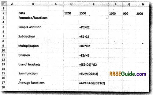
The following formulae are shown in the spreadsheet extracts shown below:
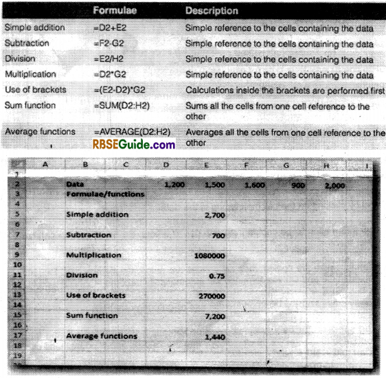
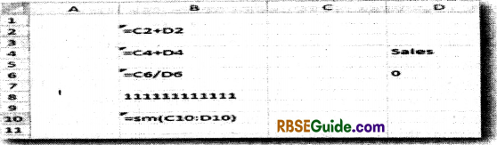
Here is the spreadhsheet again, showing the formulae behind the amounts displayed:
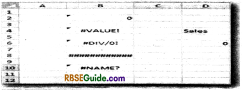
Spreadsheet Errors
Most spreadsheets have error reporting facilities. The more sophisticated tools allow formulae to be traced from cell to cell. However, even as data is entered into spreadsheet cells some errors will be reported.
In the extract below from an Excel spreadsheet, the small triangles at the top left of B2, B4 and so on indicate that there could be a problem. The second spreadsheet shows the formulae that lie behind the problem cells.
- Cell B2 contains a calculation using cells that have no values yet; C2 and D2 are empty
- Cell B4 tries to perform a calculation on a label, the word ‘Sales’
- Cell B6 tries to divide by zero (Cell D6)
- Cell B8 contents are too large to be shown in the cell. This is easily fixed by making the column wider.
- Cell B10 contains an unknown function name.
- Should be = Sum(C10 : D10)
Additionally, you might sometime, be warned about circular references. For example, if you were to enter the following in Cell C12: = C12 + D12
Then the answer to cell C12 depends on the contents of cell C12 and the spreadsheet would warn you about that, or not permit that formula to be entered.
![]()
Linking and Embedding Data from Different Sources
Often excerpts from a spreadsheet need to be incorporated into a report produced on a word processor. There are several ways in which this can be done :
1. Simple Copying: In the spreadsheet highlight the range of cells you are interested in. Press Ctrl + C to copy these. Then in the word processor document, press Ctrl + V.
This pastes a copy of the figures into the report, but there is no spreadsheet functionality there; they are just like typed figures. This can be inefficient if the spreadsheet figures change later and you have to make sure the report is brought up to date accurately.
2. Embedding : As before, copy from the spreadsheet, but select Paste Special in the word processor. This copies the selected range into the report but maintains the functionality of the spreadsheet. It’s like having a mini-spreadsheet within the report. However, there are two copies of the cells – one in the spreadsheet and one in the word processor file. These are now quite separate and changes in one will not affect the other.
3. Linking: As above but in Paste Special choose the link option. This keeps the two copies of the spreadsheet cells linked so that updating the spreadsheet can be automatically reflected in the word processor. In addition to linking spreadsheets to word processor it is possible to link several spreadsheets together. For example, there could be a spreadsheet for each of three branches, then a fourth where the results of the branches are added together.
Storing and Retrieving Spreadsheets
Selecting ‘Save’ for the first time will prompt you to enter a name for the spreadsheet. Thereafter, ‘Save’ overwrite the previous copy of the spreadsheet.
‘Save as’ allows you to select a different name for the spreadsheet. This can be useful if you want to keep several editions of the spreadsheet.
Retrieving is a simple matter of navigating to the folder where the spreadsheet was stored and clicking, or double-clicking, on it.
Most systems also provide a list of recently opened spreadsheets.
![]()
Other Use Spreadsheets
Lists: You can create lists, from shopping lists to contact lists, on a spreadsheet. For example, if you entered store items to a spreadsheet alongwith their corresponding aisles, you could sort by aisle and print before your shopping trip. Your list would provide an aisle-by-aisle overview.
The sorting power of spreadsheets becomes more evident when entering more data. Maintaining personal or professional contacts allows you to sort by every field. For example, a salesperson might enter all clients and then sort by zip code allowing him to plan his day with geographic efficiency.
Accounting : Beyond sorting, spreadsheets are invaluable calculators. By entering the appropriate mathematical functions into cells, you can turn a simple spreadsheet into an accounting page. You can list credits in one column and debits in another. The auto-sum feature speeds calculations and can be set up to maintain running totals.
And with the flexibility of spreadsheet programs, data used in equations can be anywhere on the sheet or in the workbook. Adding additional pages (sometimes called Worksheets) allows you to organise information to suit your needs. Data from anywhere in the workbook can be used in your calculations.
Time Sheets : Besides adding and subtracting integers, spreadsheets can also perform those calculations on time-based numbers. Formatting cells to reflect data as a time (as opposed to simple integers) can allow you to use the spreadsheet as a time sheet.
Additionally, you can include descriptions of assorted job functions, employee names, etc. giving you the ability to sort by those to time incurred for any of your chosen fields.
Database Use: Although, spreadsheets are not true relational databases, they can be designed and formatted to function as simplified ones. For example, if you need to track pricing of a particular product, enter its price only one time.
For all subsequent references to that price, point to the original entry as opposed to re-entering the price. When you need to change the price, change it in its original cell and all corresponding references will update automatically.
Chart Creation: Charts and graphs create better depictions of trends and percentages than raw numbers. As they say, “A picture’s worth a thousand words.” Spreadsheet programs can
automatically convert your data into the visual depiction of your choice, whether it’s a pie chart, bar chart or line graph.
There is no easy way to conduct financial forecasting. All forecasting involves the technically impossible act of predicting the future. Nonetheless, forecasting is essential for equity valuation and internal budgeting.
The best financial forecasts are educated quantitative guesses founded on a very nuanced understanding of a business, the external factors that influence business performance and forecasting techniques that typically lead to successful estimates. Assuming an analyst has intimate knowledge of a firm, its risks and catalysts, several straightforward techniques can be employed using Microsoft Excel.
Equity analysts frequently replicate financial statement data over time in an Excel spreadsheet to create a model. Each column can represent a distinct period and each row a different item on the balance sheet. This format allows analysts to observe trends over time, and other key performance metrics can easily be included to affect the model.
Such a financial model facilitates fundamental analysis and makes it easy to assess growth, margins, free cash flow, working capital management and changes to balance sheet items. Different items can be represented graphically, and all of the financial statements can flow together in a working model.
Excel can also be used for strictly quantitative forecasting when the data is appropriate. A forecast function extrapolates future values along a best fit line from univariate ordinary least squares regression. This basically takes the trendline from a two-variable scatterplot and extends it.
Excel also has an exponential smoothing function in the Data Analysis button of the Data tab. Exponential smoothing eliminates irregularities in time series data to create tease-out of an overarching trend. This trend is simply projected into future periods.
![]()
Benefits of Forecasting
Forecasting can help you make the right decisions, and earn/save money. Here is one example:
Size Your Inventories Optimally
Time is money. Room is money. So what you want to do is use all means at your disposal in order to reduce your stocks without experiencing any shortages, of course. How ? By forecasting!
How to Make Things Easy: Labels, Comments, Filenames
Over time, as your data accumulate, you will be more and more likely to get confused; to make mistakes. The solution? Don’t be messy: making good use of labels, comments and naming your files correctly can save you a lot of trouble.
- Always Label Your Columns : Use the first row of each column to describe the data it contains.
- Different Data, Different Columns: Do not put different numbers (for example, your COSTS and your sales) on the same column. It is incredibly likely for you to get confused and it makes computations and data handling more difficult.
- Give Each Tile a Clearly Understandable Name: It takes little effort and speed things up. It makes them easy to identify visually and easier to find using the windows search function.
- Use Comments : Even if you don’t usually work with a large amount of data, it is still very easy to get confused. This applies especially if you come back to the data you have created a long time before. Excel has a great solution to offer: comments.
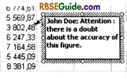
Just do a right click on the cell you want to comment, and then select « insert comment».
You can use them to explain the content of a cell (i.e., unit cost according to Mr Doe’s estimates) to leave warnings to future users of the sheet [i.e., I have a doubt about this calculation…)
Get advanced sales forecasts with our inventory forecasting web app. Lokad specialises in inventory optimisation through demand forecasting. The content of this tutorial – and much more – are native features of our forecasting engine tool.
Getting Started: A Simple Forecasting Example Using Trendlines
Viewing your data
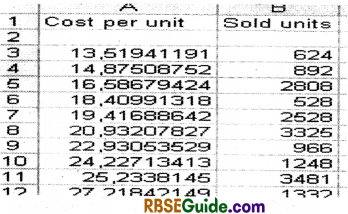
Let us now do our first forecast. In this part, we will be using this file : Examplel.xls. To repeat the steps by yourself, you can download the file. This data serves just as example.
Our Data : In the first column, data about the unit costs of similar products, (the unit cost reflects the quality of the product). In the second one, data about how much has been sold.
What We Want to Know: If we sell another product, with a quality corresponding to a cost of $150/unit, how many units can we expect to sell?
How We Get There : Here, it is pretty simple. We want to find a simple mathematical relationship between unit cost and sales, and then use this relationship to do our forecast.
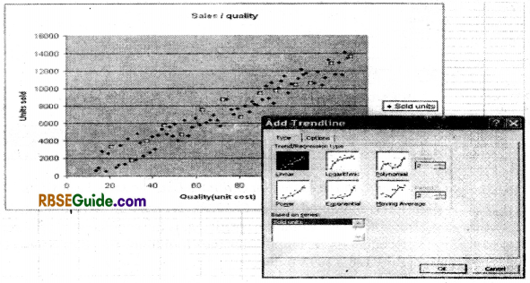
First, it is always useful to create a graph in Excel, in order to take a look at the data. Your eyes are excellent tools that can help you identifying trends in a few seconds.
To do this, we select our data, then use Insert > Chart, and choose the XY(Scatter) option. We want to estimate sales as a function of quality. Therefore, we put the unit cost on the horizontal and the sales on the vertical axis.
Now, we stop a few seconds and take a good look at what we see : the relationship seems to be increasing and linear.
In order to get an idea of the exact form of the relationship. We right click on the chart and select the “Trendline” option.
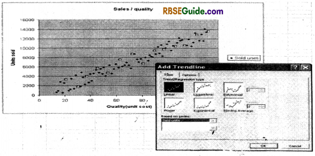
Creating a trendline
Now, we have to select the relationship that seems to “fit” (i.e., best describe) our data. Here again, we use our eyes: In this case, the dots are almost in a straight line, so we use the “linear” setting. Later on, we will use other – more complex, but often more realistic – settings, like “exponential”.
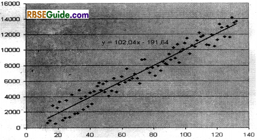
Our trendline is now displayed on the chart. Another right click allows us to display the exact form of the relationship: y = 102.4x – 191.64.
Understand: Number of units sold = 102.4 times the unit cost – 191.64.
So, if we decide to produce at a $150 unit cost, we can expect to sell 102.4*150 – 191.64 = 15168 units.
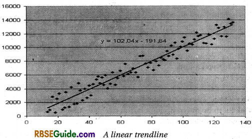
A linear trendline
We have just completed our first forecast successfully.
However, be careful: The software is always able to find a relationship between the two columns, even if this relationship is in reality very weak. Therefore, a check for robustness is required. Here is how you quickly do this:
First, Always Take a Look at the Chart: If you find the dots closely located to the trendline, as is the case in our example above, there is a good chance that the relationship is robust. However, if the dots seem to be located almost randomly and are in general quite far from the trendline, then you should be careful : the correlation is weak, and the estimated relationship should not be blindly trusted.
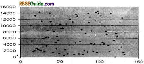
The dots are everywhere : no evident relationship, unrealiable forecasts.
After taking a look at the chart, you can use the CORREL function. In our example, the function would read: CORREL (A2:A83,B2:B83). If the result is close to 0, then the correlation is low, and the conclusion is: there is simply no real trend. If it is close to 1 then the correlation is strong. The latter is a helpful, since it increases the explanatory power of the relationship you found.
There are more subtle ways of making sure the correlation is high; we will come back to this later on.
Of course, these last steps can be automated : you don’t have to note the relationship, and use your pocket calculator to do the computation. You need the Analysis Toolpak!
![]()
Forecasting Using the Analysis Toolpak
Before proceeding, you should check if the Excel ATP (Analysis Toolpak) is installed. Refer to the section Installing the Analysis Toolpak, for further information.
Unfortuntaley such perfect sales data with such a nice, simple linear relationship is quite uncommon in real life. Let us have a look at what Excel has to offer for more complicated situations, with more complicated data.
![]()
Going Further: The Example of Exponential Fitting
As you might imagine, such a linear model of your data is not always likely. In fact, there are many reasons to believe that it should follow an exponential model. Many behaviours in the economy are driven by exponential equations (i.e., Interest compounding computations are a classical example).
Here is how to perform an exponential fitting :
1. Take look at your data. Draw a simple graph, and just look at it. If they follow an exponential evolution, they should look like this

Perfect exponential shape
This is the perfect case, of course, the data will never exactly look like this. But if the dots seem to approximately follow this repartition, it should encourage you to consider exponential fitting.
Using trendlines
As in the previous example, you can always draw a chart of your data, ask for a trendline, and choose « exponential» instead of linear. Then, gather the displayed equation, as usual.
2. Luckily, you can also do all this directly, using the Analysis Toolpak. Put all your data into a blank excel sheet, and go to Tools => Data Analysis.
![]()
Installing the Analysis Toolpak (ATP)
The ATP is an add-ui that comes with Microsoft Excel, but that is not always insta’led by default. In order to install it, one can proceed as follows:
Make sure you have your Office CD with you. Excel might require you to insert the CD in order to install the AlP files
1. Open an excel sheet, and go to Tools Menu, and then select Add-Ins. Check the first box of the window, labelled « Analysis Tolpak »
2. Insert your Office CD if asked to do so by the software.
3. That’s it! Notice that your « Tools)) menu now includes many more features, including a « Data Analysis» option. This is the one that we will use the most.
Using the Analysis Toolpak (ATP) … in a Linear Setting
Now, let us come back to our linear example. If your data « looks » good (see above illustration),
you can use the ATP to get a direct estimation of the functional form, without going through the
«trendiine »process.
Open your data sheet, then open the « tools » menu and select « Data Analysis ». A window pops up, asking you what kind of analysis you want to perform, Select regression» for linear settings.
Now you need to give Excel two arguments: an « Y range » and an « X range ». The Y range indicates what you want to estimate (i.e., your sales), and the X range contains the data that you think can explain your sales (here, your unit cost). In our example (see example 1 .xls), our sales data are in column B, from row 3 to row 90, so you need to put « $8$3:$8$90 » as the Y range, and «$A$3:$A$90 » as the X range, when you are done, click « ok ». A new sheet appears, containing the « regression results ».
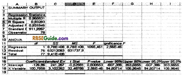
The Analysis Toolpak Output, in the case of an Ordinary Least Squares Regression. The most important result is contained in the « Coefficients » column at the bottom of the sheet. The intercept is the constant, and the « X variable » coefficient is the coefficient of X (here, your unit cost). Hence, we find the same equation we found using the « trendline » function. Sales = Intercept + Xcoefficient * unit cost Sales = – 126 + 1oo * unit cost.